LoRA: Low-Rank Adaptation of Large Language Models

"LoRA: Low-Rank Adaptation of Large Language Models" 논문을 한국어로 정리한 포스트입니다.

LoRA: Low-Rank Adaptation of Large Language Models

Edward Hu, Yelong Shen,
Phillip Wallis, Zeyuan Allen-Zhu, Yuanzhi Li, Shean Wang, Lu Wang, Weizhu Chen

 

Introduction

---

Terminologies

• $d_{model}$: Transformer 레이어의 입력 및 출력 차원 크기
• $W_q$, $W_k$, $W_v$, $W_o$: self-attention 모듈에서 query, key, value, output projection 행렬
• $W$ 또는 $W_0$: 사전 학습된 가중치 행렬
• $\Delta W$: Adaptation 중에 누적된 기울기 업데이트
• $r$: LoRA 모듈의 rank

Problem Statement

---

• $P_{\Phi}(y\mid x)$ → $\Phi$ 로 paramerized 된 pretrained model
• $\mathcal{Z} = \{(x_i,y_i)\}_{i=1,\cdots,N}$
• → downstream task의 context($x$)-target($y$) 쌍의 학습 데이터셋
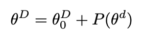
• fine-tuning 중 모델은 $\Phi_0$ 으로 초기화된 후, 아래의 objective function을 최대화 하기위해 gradient를 따라 $\Phi_0 + \Delta\Phi$로 반복적으로 업데이트 됨

$$ \underset{\Phi}{\max} \underset{(x,y) \in \mathcal{Z}}{\sum}\underset{t=1}{{\overset{\left| y\right|}{\sum}}}\log(P_{\Phi}(y_t\mid x,y_{<t})) $$

• fine-tuning의 주요 문제는 각 task에 대해 $\left|\Delta\Phi \right|$ 와 $\left|\Phi_0 \right|$ 가 같다는 점 ( = 모든 parameter가 학습에 포함됨, GPT3의 경우 $\left|\Delta\Phi \right| \approx$ 1750억)
• → 각각의 fine-tuning된 모델에 대해 독립적인 인스턴스를 저장하고 배포하는 것은 매우 어려운 일
• 본 논문에서는 더 parameter-efficient한 접근 방식을 사용.
  • task-speific 한 parameter 변화량 $\Delta\Phi = \Delta\Phi(\Theta)$ 이 훨씬 작은 size의 $\Theta$로 인코딩 ( $\left|\Theta\right| \ll \left|\Phi_0 \right|$ ).
  • $\Delta \Phi$를 찾는 과정이 아래와 같이 $\Theta$로 최적화할 수 있게 됨.
  $$ \underset{{\color{Red}\Theta}}{\max} \underset{(x,y) \in \mathcal{Z}}{\sum}\underset{t=1}{{\overset{\left| y\right|}{\sum}}}\log(P_{{\color{Red}\Phi_0+\Delta\Phi(\Theta)}}(y_t\mid x,y_{<t})) $$

 

Intrinsic Dimension 수식과 비교

• 본 논문에서는 $\Delta \Phi$ 를 encode할 수 있는 low-rank representation을 제안함.
  • GPT3 기준 $\left|\Theta\right|$ 는 $\left|\Phi_0 \right|$ (175B)의 0.01%

Aren’t Existing Solutions Good Enough?

---

• Transfer learning 이후 모델 adaptation을 효율적으로 하고자한 시도는 계속 있었음. 크게 두가지 전략 존재
  1. Adapter 레이어 추가
  2. Optimizing some forms of the input layer activations (prefix tuning)

1. Adapter Layers Introduce Inference Latency

• Adapter 변형 방식은 다양하지만 다음 2가지를 주로 체크
  1. Transformer block 당 두 개의 adapter를 사용하는 디자인 (by Houlsby et al. (2019)) $Adapter^H$
  2. 블록당 하나만 있지만 LayerNorm을 쓰는 경우 (by Lin et al. (2020)) $Adapter^L$

Adapter layer는 매우 적은 parameters (가끔은 original model의 1% 이하)를 쓰기 때문에 큰 문제로 보이지 않을수 있지만, large neural networks는 latency를 낮추기 위해 Hardware parallelism에 의존하며, adapter layer는 순차적으로 처리됨. → 이는 batch size가 1에 가까운 online inference 환경에서 차이를 만듬.

2. Directly Optimizing the Prompt is Hard

• prefix tuning은 최적화가 어려우며 performance가 non-montonically하게 변함.
• 근본적으로, adaptation을 위해 입력 sequence의 일부를 점하는 것은 downstream task에서 사용가능한 sequence 길이를 줄이고, 이로 인해 prompt를 tuning하는게 다른 방식들에 비해 성능이 떨어지는걸 봐왔음.

Our Method

---

1. Low-Rank-Parametrized Update Matrices

• 신경망은 matrix multiplication을 하는 수많은 dense layer들로 이루어져 있고, 이러한 layer의 weight matrix들은 일반적으로 full-rank를 가지고 있음

Intrinsic Dimensionality Explains the Effectiveness of Language Model Fine-Tuning

• 특정 task에 adpatation할때, pre-trained language model은 훨씬 적은 ‘intrinsic dimension’을 가지고 있고, 더 작은 subspace하게 random projection 하는 것만으로도 효율적으로 학습할 수 있음.

Inspired by this, we hypothesize the updates to the weight also have a low “intrinsic rank” during apdatation

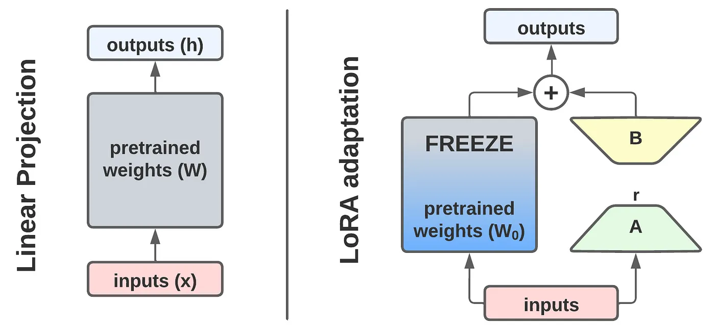
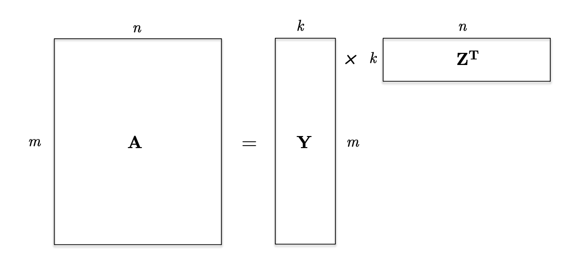
• 사전 학습된 weight matrix $W_0 \in \mathbb{R}^{d \times k}$, update 값 $\Delta W$를 low-rank decomposition $BA$로 대체함.</aside>

  Matrix Weight $W$의 변화량($\Delta W$)값을 low rank로 간소화!

$$ W_0 + \Delta W = W_0 + BA \quad where \; B \in \mathbb{R}^{d \times r},\; A \in \mathbb{R}^{r \times k} \quad (\,r \ll \min(d,k)\,) $$

 

• $W_0$는 freeze, $A$와 $B$는 학습 가능한 paramter. $h=W_0x$일 경우, 변경된 forward pass는 다음과 같음

$$ h = W_0x + \Delta Wx = W_0x + BAx $$

 

• We use a random Gaussian initialization for $A$ and zero for $B$, so $∆W = BA$ is zero at the beginning of training. We then scale $∆W x$ by $α\over{r}$, where $α$ is a constant in $r$. When optimizing with Adam, tuning α is roughly the same as tuning the learning rate if we scale the initialization appropriately.

 

 

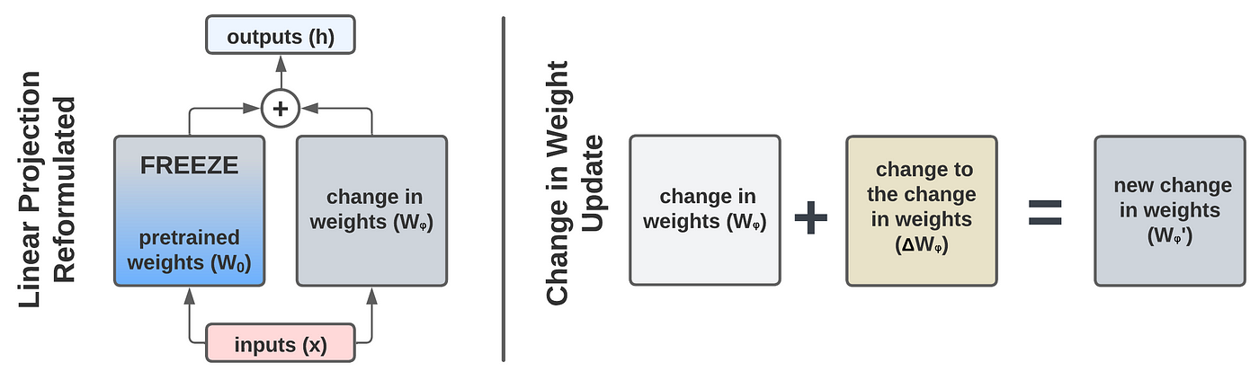
A Generalization of Full Fine-tuning

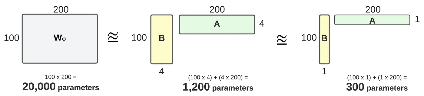
Comparison of rank-4 and rank-1 adaptation. LoRA results in fewer trainable parameters.

BA as an approximation of the change-in-weight matrix (Wᵩ).

• LoRa는 가중치 행렬이 full-rank로 gradient update될 필요가 없음.
• rank $r$ 이 pre-trained matrices와 유사하게 설정할 경우 전체 fine-tuning과 같은 expressiveness를 복구할 수 있음 .
  • Adapter 방식은 layer가 추가되고, prefix 기반 방식은 입력 시퀀스가 제한되기 때문에 원래의 finetuning으로 수렴될 수 없음.
• → 학습되는 parameter 수가 증가할수록 LoRA는 원래의 finetuning 방식으로 수렴

No Additonal Inference Latency

• production 환경에서 $BA$ 만 변경하는 방식으로 다른 downstream task로 전환이 간편함.
• 결정적으로 adapter기반 방식들에 비해 inference시 추가적인 latency가 없음

 

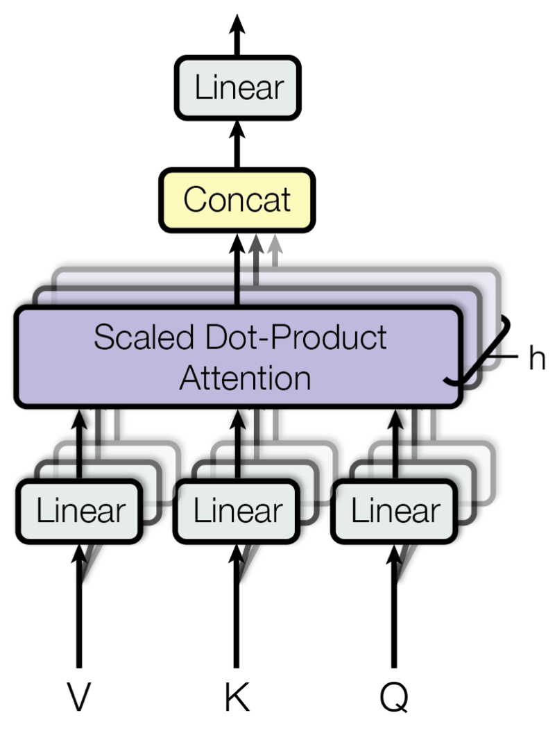
2. Applying LoRA to Transformers

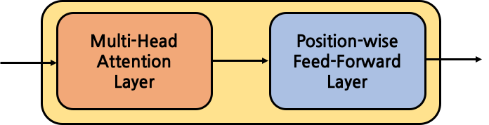
• 이론적으로, LoRA는 신경망 내의 어떤 weight matrices라도 적용이 가능하며, 학습 가능한 parameter를 줄여줄 수 있음.
• Transformer 구조에서 attention module에는 4개의 weight matrices ($W_q, W_k,W_v,W_o)$가 존재하고 MLP module에는 2개가 존재함.
• 본 논문에서는 attention weights에만 적용. MLP module은 학습되지 않음.4 weight matrices in attention module

Empirical Experiments

baseline

Validation Accuracy vs. number of trainiable parameters

Understanding the low-rank updates

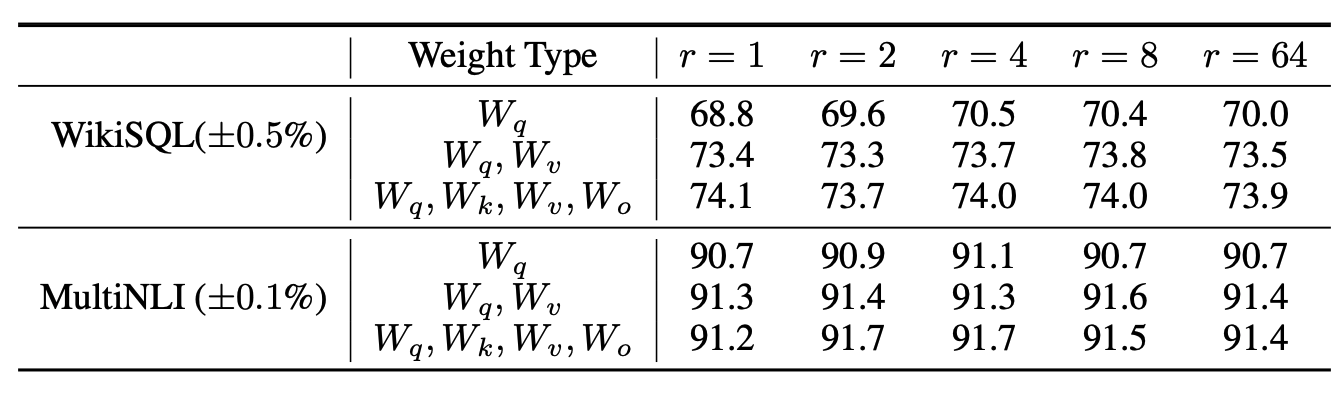
Which weight matrices in transformer should we apply LoRa to?

• putting all the parameters in $\Delta W_Q$ or $\Delta W_k$ results in lower performance, adapting both $W_q$ and $W_v$ yields the best result.
• 하나의 weight에 더 큰 rank로 adapt하는 것 보다, rank가 적더라도 더 많은 weight matrices를 쓰는게 더 좋음

What is the optimal rank $r$ for LoRA?

• 매우 작은 $r$로도 충분한 성능을 보여줌.
• 이는 $\Delta W$ 를 업데이트 하는게 매우 작은 ‘intrinsic rank’ 를 가지고 있음을 의미함.
• → 물론 작은 $r$이 모든 task에 대해 작동한다는 것은 아님. 2개의 다른 언어로 구성된 downstream task가 있다고 했을 때, pre-train이 한 언어로 만 진행되었다면, 전체 모델을 retraining하는 것($r=d_{model}$)이 작은 $r$ 의 LoRA로 학습하는게 확실히 더 좋은 성능을 보일 것
• $r$을 증가시키는게 더 많은 의미 있는 subspace를 cover하지 못한다면, 낮은 랭크의 adaptation matrix로 충분하다고 볼 수 있음

 

Preliminary

Singualr Value Decomposition (SVD)

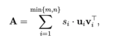
1. SVD 는 matrix $A$ 를 “list of its ingredients”로 나타낸 것으로 볼 수있음.

→ SVD는 A를 $min \{m,n\}$ 개의 rank-$1$ matrices의 linear combination 으로 표현한 것과 같음. (일치하는 signular values들로 weighted 되는)

1. 모든 matrix는 SVD를 가지고 있음
2. Geometrically, $U,V^\top$ 는 rotation을, $\Sigma$ 는 scaling을 수행함.

Low Rank Approximation

• General Definition : $k$개의 rank-$1$ matrices의 합으로 표현 가능한 matrix의 rank는 $$ $k$임.
• $A$를 표현하는 최적의 rank-$k$ 를 찾는다
  • 만약 matrix $A$ 를 성분(ingredients)의 합으로 표현(representation)할 수 있고, 이 성분들이 중요도(importance)순으로 정렬되어 있다면, 가장 중요한 $k$ 개를 가져와 rank $k$ matrix로 approximation 할 수 있다.
  • → SVD 가 정확하게 같은 representation을 제공 : SVD
  • The rank-$k$ approximation is then,

$$ A_k = U_kS_kV_k^\top $$

Low rank approximation via SVD

Frobenius Norm

• Frobenius norm은 singular value의 L2 norm 과 같음

$$ \lVert A \rVert_F = \sqrt{ \sum_{k=1}^n \sigma_i^2} $$

Subspace similarity between different $r$

1. $A_{r=8}, A_{r=64}$ : $r$ = 8, = 64 로 학습한 모델 (with the same pre-trained model)
2. Low rank approximation 계산을 위해 SVD 계산후 top $k$ 를 계산

• singluar value decomposition을 통해 right-singular matrices $U_{A_{r=8}}, U_{A_{r=64}}$를 계산

How much of the subspace spanned by the top $i$ singular vectors in $U_{A_{r=8}}$ (for $1\le i \le 8$) is contained in the subspace spanned by top $j$ singular vectors in $U_{A_{r=64}}$ (for $1\le i \le 64$)?

• Grassmann distance를 기반으로한 normalized subspace similarity 식 
  • $U_A^i \in \mathbb{R}^{d\times i}$, $U^i_A$ = columns of $U_{A_{r=8}}$ corresponding to top-$i$ singular vectors
  • $\phi(\cdot)$ → 1 = complete overlap of subspaces / 0 = a complete sepration

 

추가 설명

• rank에 관계 없이 같은 pretrained model 이라면 $\Delta W$는 동일한 형태며 $d \times d$ 의 형태라고 가정
• $U_A^i \in \mathbb{R}^{d \times i}, U_B^j \in \mathbb{R}^{d \times j}$
• ${U_A^i}^\top U_B^j$ $\in \mathbb{R}^{i\times j}$ 의 singular value를 $\sigma_1 \cdots \sigma_p (p = min(i,j))$라고 했을때, Ham & Lee (2008) 이 제안한 distance는 다음과 같음

• 위 식을 기반으로 본 논문에서 제안한 similarity는 다음과 같이 표현 가능
  • $d(\cdot) = 0$ → $\phi(\cdot) = 1$ → $U_A, U_B :$ similar
  • $d(\cdot) = \sqrt{p}$ → $\phi(\cdot) = 0$ → $U_A, U_B :$ orthogonal

 

 

• $\Delta W_v$ of $A_{r=8}$ and $\Delta W_v$ of $A_{r=64}$ share a subspace of dimension 1 with normalized similarity > 0.5
• → why $r=1$ performs quite well.
• top singular-vector direction are most useful. While other directions potentially contin mostly random noises accumulated during training.

Subspace similairity between different random seeds

• plotting the normalized subspace similiarity between two randomly seeded runs with $r=64$

• $\Delta W_q$ appears to have a higher “intrinsic rank” than $\Delta W_v$
  • more common singular value directions are learned by both runs for $\Delta W_q$
• 2 random Gaussian matrices do not share any common singular value directions with each other.

실험 분석 결론

• apdatation matrix는 사실 매우 낮은 rank를 가지고 있음
• $\Delta W_Q$가 $\Delta W_v$보다 더 높은 intrinsic rank를 가지고 있음.

How does the adaptation matrix $\Delta W$ compare to $W$?

• Does $\Delta W$ highly correlate with $W$?
• How “large” is $\Delta W$ comparing to its corrsponding dicrections in $W$?

To answer this question

• project $W$ onto $r$-dimensional subspace of $\Delta W$ by comupting $U^\top W V^\top$
  • $U/V$ being left/right singular-vector metrix of $\Delta W$

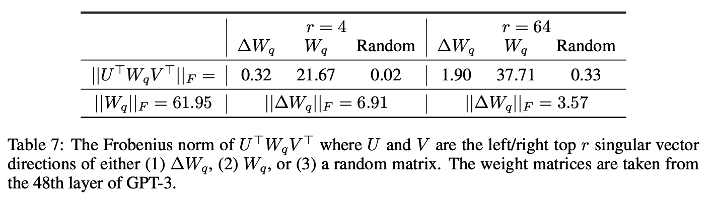
• Compare the Frobenius norm between $\lVert U^\top W V\top \rVert_F$ and $\lVert W \rVert_F$
  • we can consider a feature amplication factor = $\frac{\lVert \Delta W \rVert_F}{\lVert U^\top W V^\top \rVert_F}$
    • $U^\top W V^\top$ = projection of $W$ onto the subspace spanned by $\Delta W$
    • $\lVert \cdot \rVert_F$ = sigular value의 L2 Norm
      • sigular value는 matrix에서 scaling 값을 의미함
  • $\Delta W$ 가 task-speific 한 direction을 내포한다고 했을때, amplication factor는 기존의 $W$ 가 얼마나 증폭됐는지를 의미함.
  • Amplication factor
    • $r=4$: $21.5 \approx 6.91/0.32$
    → there are four feature directions in each layer (out of the entire feature space from the pre-trained model $W$), that need to be amplified by a verly large facotr 20, in order to achieve our reported accuracy.
    • $r=64$: $2 \approx 3.57/1.90$
    → Most driections learned are not being amplified by much.
  • → the intirinsic ranck needed to represent the “task-speific directions” is low.

conclusion

1. $\Delta W$ has a stronger correlation with $W$ compared to random matrix
2. → $\Delta W$amplifies some features that are already in $W$
3. Instead of repeating the top singulare directions of $W$, $\Delta W$only amplifies directions that are not emphasized in $W$

The low-rank adaptation matrix potentially amplifies the important features for specific downstream tasks that were learned but not emphasized in the general pre-training model

 

Conclusion

• LoRA, an efficient adaptation strategy that neiter introduces inference latency nor reduces input sequence length while retaining high model quality.
• It allows for quick task-switching when deployed as a service b6y sharing the vast majority of the model paramters.
• We focused on Trasnformer language models, the proposed principles are genrally applicable to any neural networks with dense layers.